Mar

Jan
19
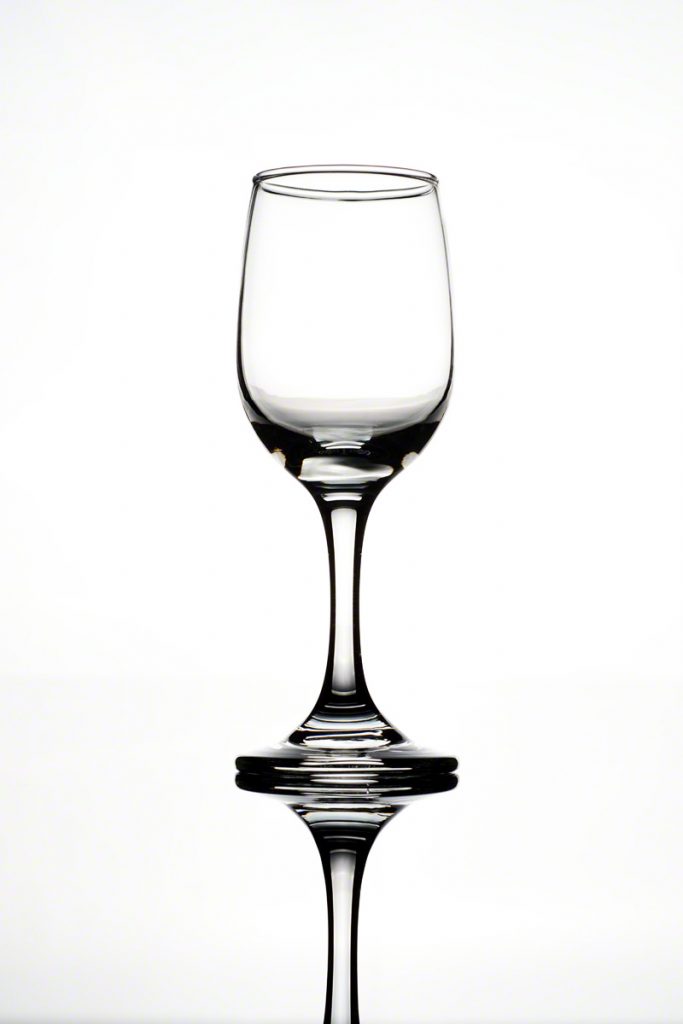
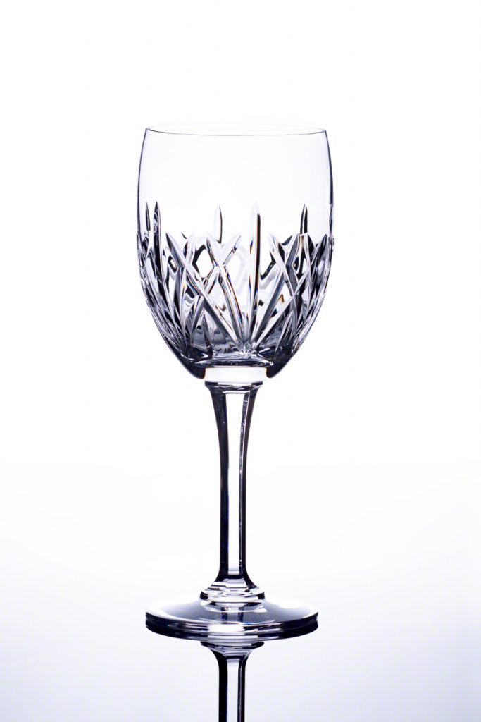
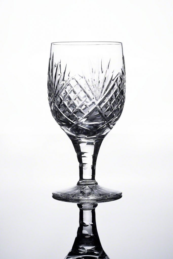
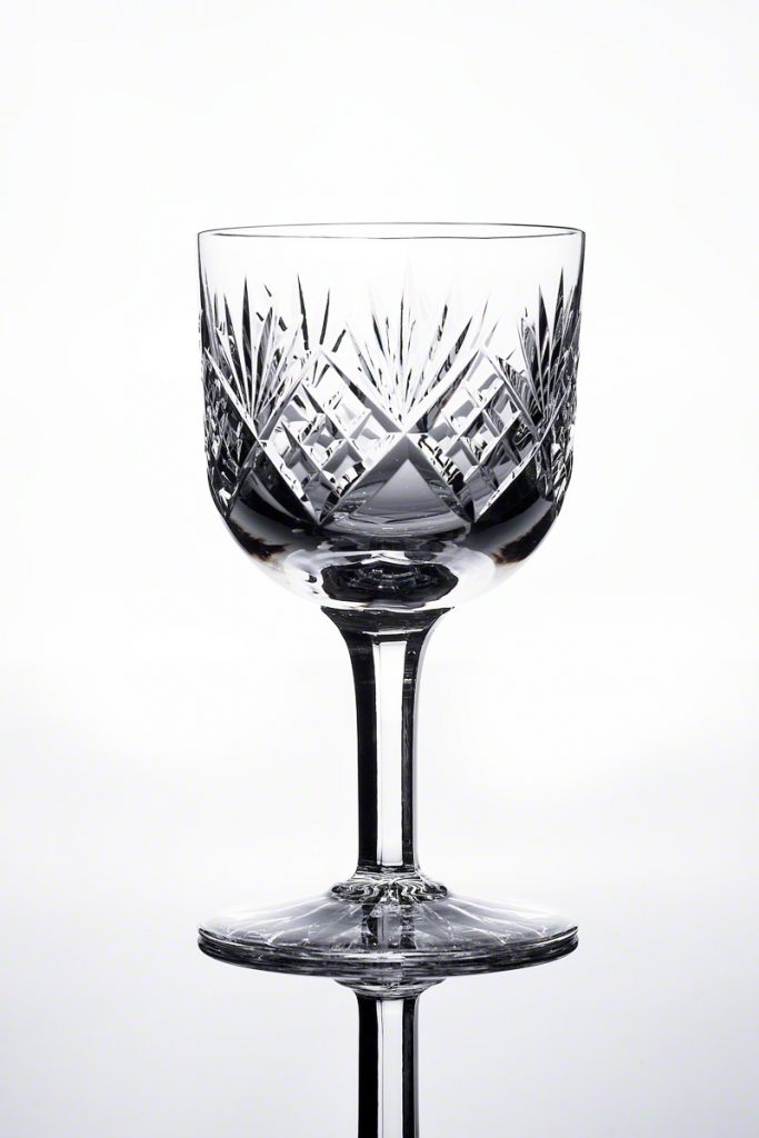
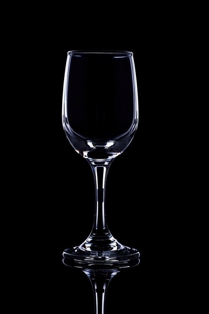
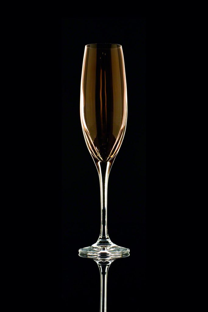
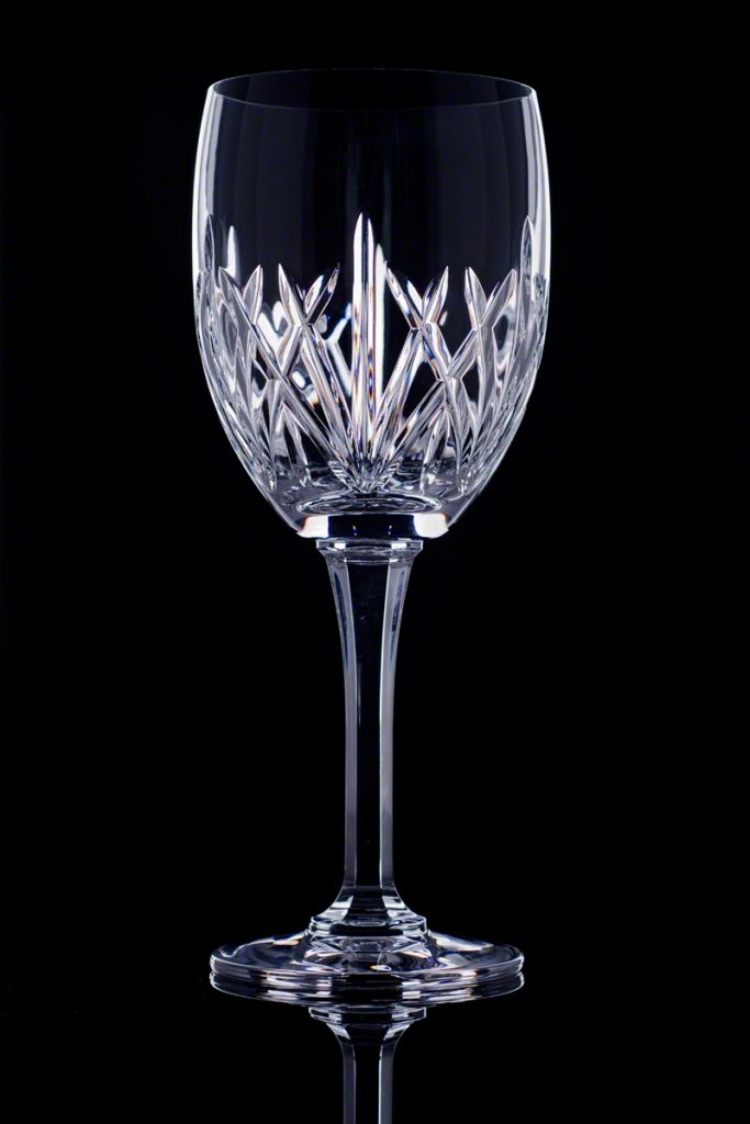
Having not posted for a while, and having recently paid my annual fees, it seemed appropriate to raise a glass to theDoctorsImages by posting some images of, well.., glassware. Items with high translucency and high reflectivity can be difficult to shoot cleanly, and there are various techniques with which to do this. Here I used a simple softbox to backlight or rimlight the subject, with either the white or black background, according to which look I wanted. The glasses rest on a black plexiglass sheet in all cases. The high-key images have black foam core reflectors on either side (just out of shot) and the low-key images have white foam core reflectors either side, again, just out of shot.
The images were taken using a Fujifilm XT-2 with a Nikkor 60mm Macro Lens and a single Nissin i60 (for Fujifilm) speedlight in an inexpensive Neewer Strip Softbox. Raw file editing was performed using Alienskin Exposure X4 with finishing and sharpening in Adobe Photoshop.
Gallery

Jun
03
Super-Resolution Imaging using a Fujifilm XT-20
Cameras / Computing / Fujifilm XT-20 / Photography / Super-Resolution Photography Posted by Robin
/
0 comments
Super-Resolution
Overview of Super-Resolution Techniques, What are we Discussing Here?
Super-resolution is a term with many modern meanings, but basically involves those techniques which add detail to poor resolution and grainy images. Fractal techniques for enlarging images have existed for many years, but are really just retaining existing detail, during enlargement, in a plausible way. More modern, single image, techniques however, can actually add extra detail that wasn’t there to begin with. Some techniques work by creating a dictionary of low resolution parts (for example in facial recognition) in which similar details are found (for instance an eye or a mouth) and patched together to form a complete picture. These new, but similar, parts are then substituted for higher resolution examples of the same details to create a higher resolution image overall. Whilst ingenious, this is a step removed from using the information within the image itself directly and not the subject of this discussion.
Another technique is known as resolution-stitching. In this technique a series of close-up images from a wider scene are taken and stitched together to make a higher-resolution whole. Taking the example of a landscape image, perhaps taken with a 24mm lens. The scene would be re-shot with a longer lens, say 100mm, in such a way that you have overlapping patches which can be stitched together using appropriate software. The longer the lens, the more detailed the final image will be. This is essentially the same as panorama photography and is also not the topic of this discussion. For the sake of completeness, when considering resolution stitching, there is a related technique attributed to the Wedding Photographer Ryan Brenizer called the Brenizer technique or sometimes the Bokeramah technique. This uses a telephoto lens, opened up to give a narrow depth of field, to take overlapping images to include the background such that the subject is very sharp but the background is blurred out, yet remains relatively wide angle. See Ryan in action via this B&H interview and video.
Finally, there are also artificial intelligence (AI) systems using a variety of neural networks and so-called deep learning which are also able to fill in missing detail in a range of images. One recent, well-known, example is Google’s RAISR (Rapid and Accurate Image Super Resolution) system as seen in this 2-minute papers video. For the interested reader there are a range of videos on neural networks in the YouTube Computerphile channel.
So what am I talking about? I’m talking about the super-resolution technique for photography popularised by Ian Norman from the photon collective in 2015. Take a look at Enhance! Superresolution Tutorial in Adobe Photoshop on YouTube and Ian’s excellent Peta Pixel piece A Practical Guide to Creating Superresolution Photos with Photoshop for more information on the technique and how it is applied.
Experiments with Super-Resolution
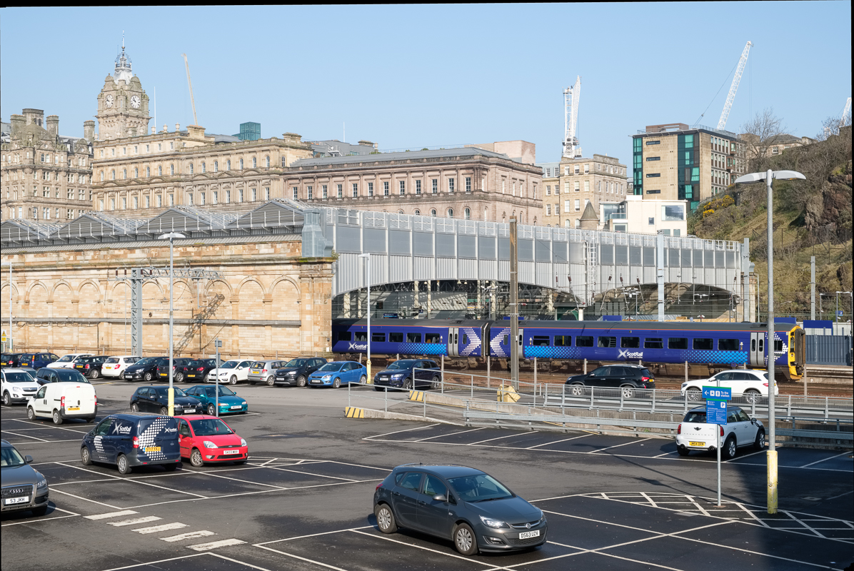
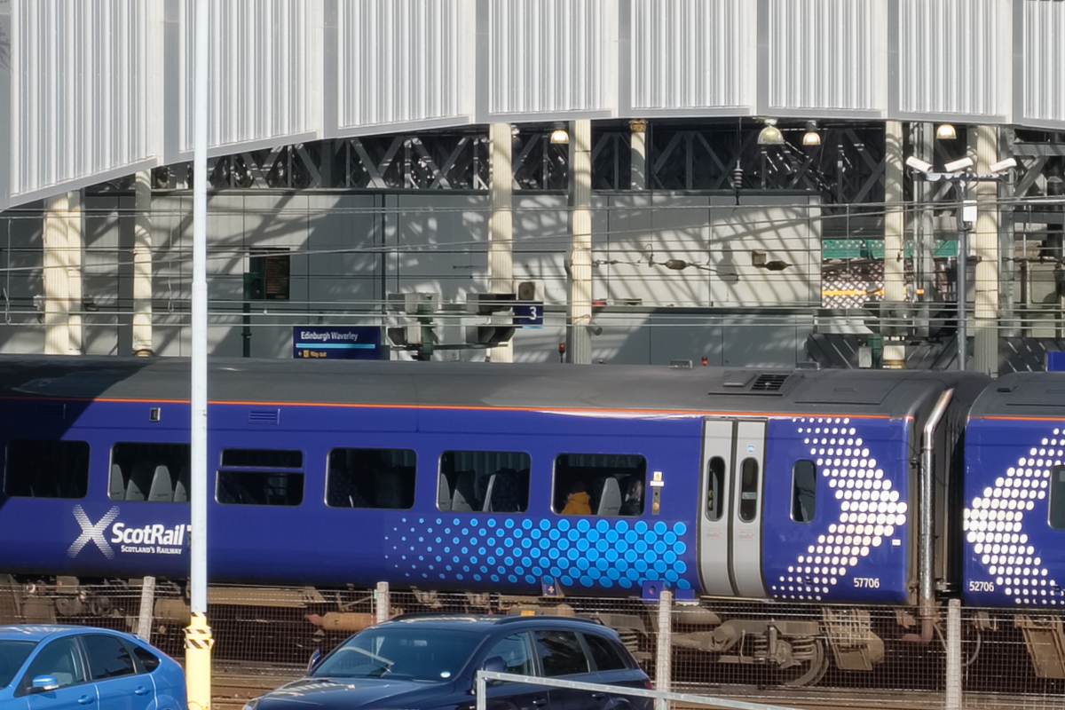
There’s little sense in me re-creating Ian’s work here, so I’ll move straight into my immediate reflections on reading his articles on super-resolution myself. I was away in Edinburgh for a long weekend and my immediate reaction was “I’ve got to try that!!” and “I wonder whether it will work with an X-Trans sensor camera” as I had my XT-20 with me. Only one way to find out, so I took a few random image bursts by way of experimentation.
Why the Worry About X-Trans?
I’ve read a great deal about the X-Trans sensor and am not sure what to make of the very partisan portrayals sometimes seen. From my own practical experience, I don’t find that the x-trans files are as easy to process when the shooting conditions have been difficult, and sharpening is often an issue unless you remember the tricks.
- Use Iridient X-Transformer to demosaic or..
- Turn off sharpening in Lightroom altogether, convert to a .tiff, then sharpen back in Lightroom or in Photoshop or..
- If sharpening in Lightroom has to be done, use the detail slider not the amount slider or..
- Use a different raw processor such as Capture One or On1 Photo Raw.
But actually, my concern was more about the green blocks of 4 pixels in the matrix. Would this effect the pixel averaging that takes place in the super-resolution process resulting in lower resolution than with a Bayer sensor? Would there be as much sub-pixel information available? This is the sort of situation where a little knowledge might be dangerous.
An Insight Into Sub-Pixel Imaging
I find it quite difficult to imagine how information can be gathered at a sub-pixel level when it is only captured at a pixel level. Looking into the research on image processing however, there are lots of different ways of extracting this information, even from a single image.
This paper by John Gavin and Christopher Jennison from 1997 called ‘A Subpixel Image Restoration Algorithm‘ gives a useful insight to the theory and practise. Indeed there are many applications in common usage including processing images of landscapes, remote sensing of active volcanos, locating and measuring blood vessel boundaries and diameters etc.
But will Ian’s process really reveal more detail, or simply smooth out the imperfections (noise) whilst placing the image on a larger canvas? Time for an experiment to find out whether super-resolution is a viable technique on X-Trans sensor cameras.
Technique
I used my Fujifilm XT-20 in manual shooting mode. The exposure was 1/250 second at an aperture of f8.0 for maximum sharpness. I used the highly respected ‘kit’ lens 18-55mm f2.8-4.0 set at 32.9mm. Several bursts of 25 images were taken, hand-held. For post processing I used Ian’s technique via specially constructed actions for 200% and 400% super-resolution. The original raw files were processed in Lightroom Clasic v7.3.1 using Auto settings, Camera ASTIA/Soft profile and the as shot auto white balance setting. Iridient X-Trans conversions were performed from within Lightroom. Final sharpening of the images was done via smart-sharpen with a setting of 300% at a radius of 2 pixels and no noise reduction. Detail shots were resized from the super-resolution images to 1200 by 800 pixels and saved via Lightroom’s export function as jpeg’s at 100% quality.
Image Results
Given the potential for artifacting in Lightroom, I generally demosaic special images in Iridient X-Transformer which, except for a single comparison just to see if there would be any difference, was the case here. So the Fuji raw files were demosaiced using X-Transformer prior to enlarging, aligning and then averaging using a smart object stack mode of mean. 5, 10, 15 and a full 25 images were enlarged to either 200 or 400%. Post enlargement, mild sharpening was applied using Smart Sharpen set at Amount 300, Radius 2 px and Noise Reduction 0%. Illustrative details from the scene are compared below. Representative details of the overall scene were selected and down-sampled to 1200 x 800 pixels for this section. This might not be the best way to demonstrate the improvements achieved by the super-resolution blending, but it does allow us to compare like with like.
Comparison results are set out as follows:
- Differences between Lightroom and Iridient X-Trans Demosaicing for the single image result.
- Differences between the 25 Image Blend at 200% size (96 mega-pixel equivalent) for Lightroom and Iridient X-Trans Demosaicing.
- 25 Image Blend at 400% (384 mega-pixel equivalent, Iridient X-Trans Demosaicing only).
- 200% and 400% with a 15 Image Blend.
- 200% and 400% with a 10 Image Blend.
- 200% and 400% with a 5 Image Blend.
- Please note that all blended shots are uncropped.
Single Image Results
Lightroom Demosaicing
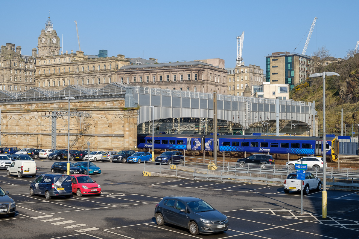
Waverley Station, Single Image..

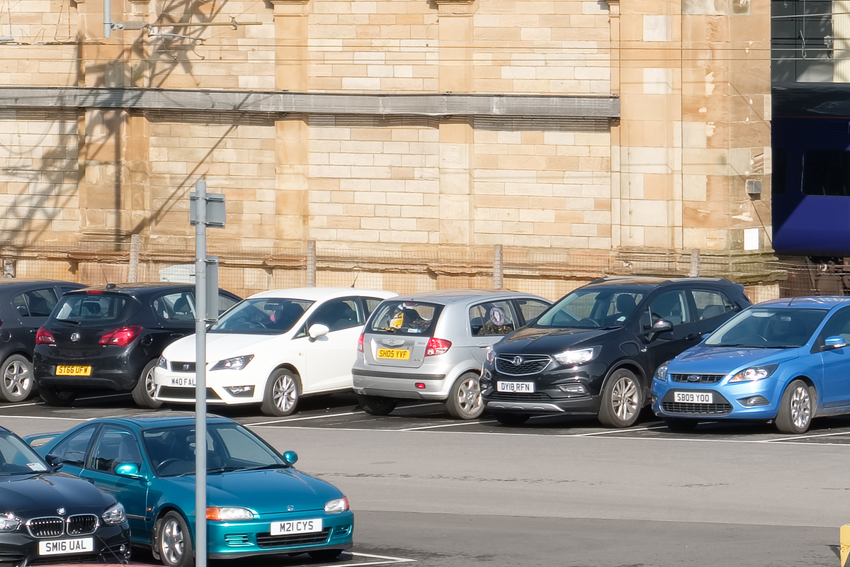
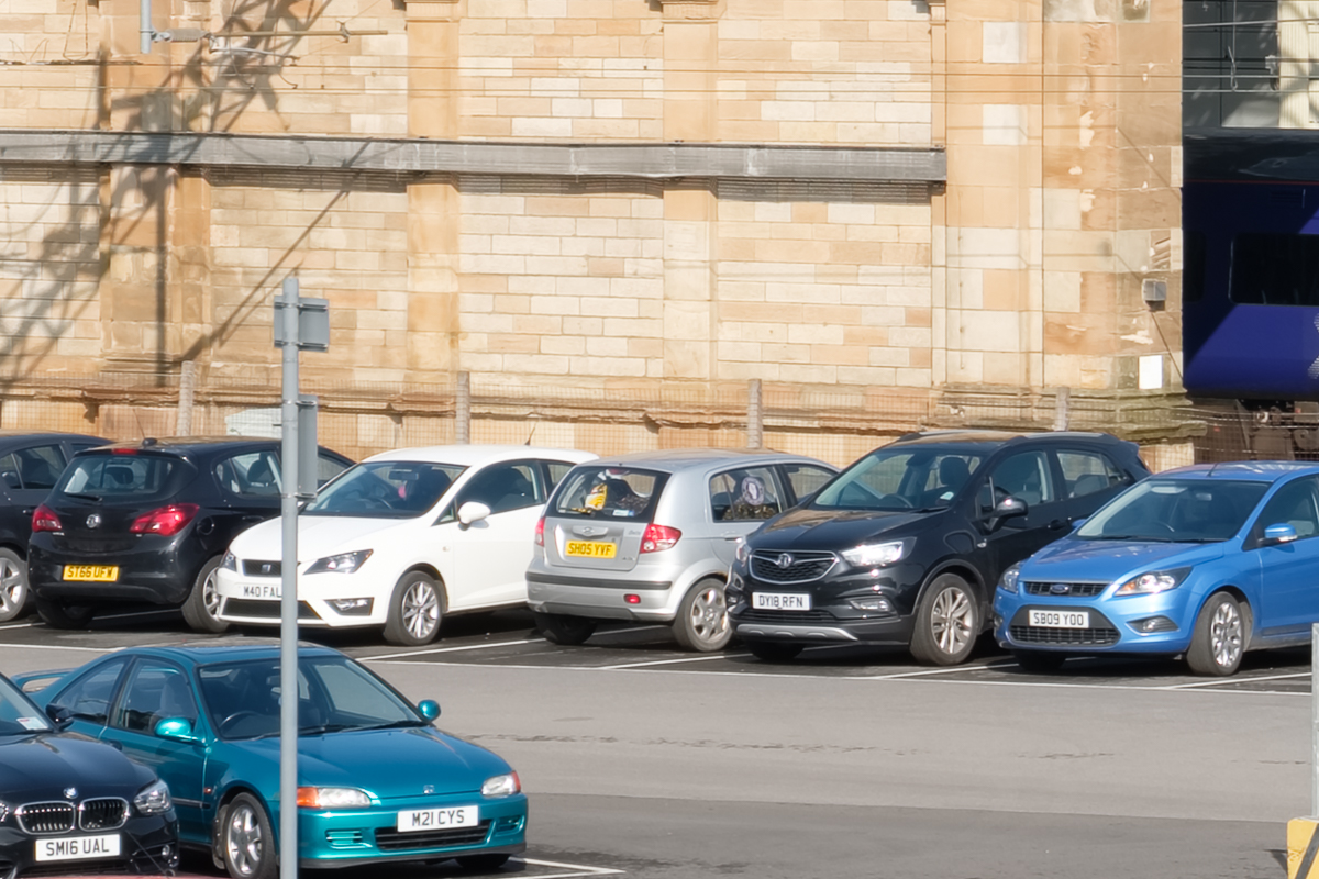
Car Detail..
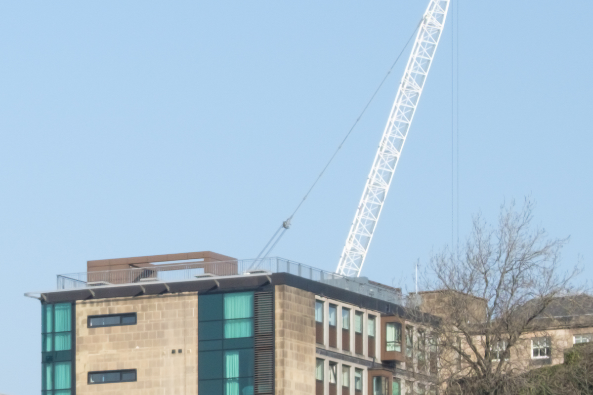
Crane Detail..

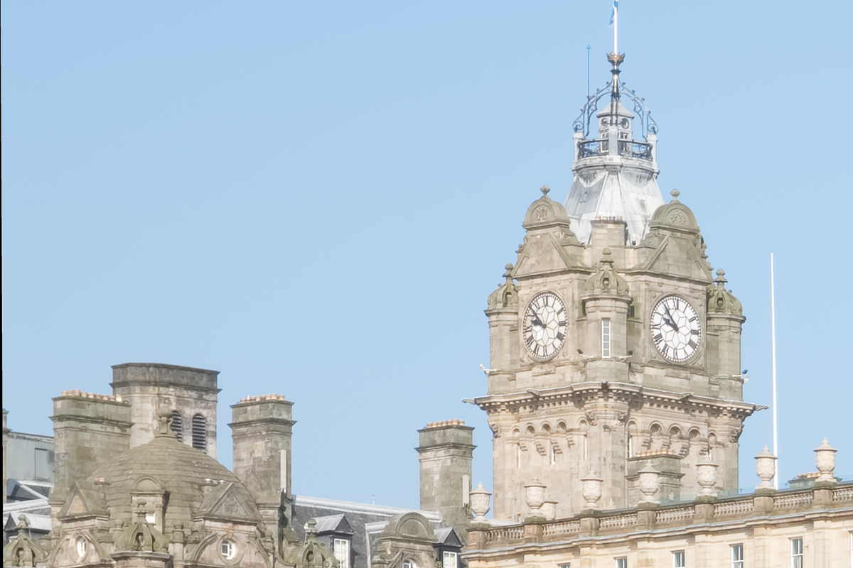
Clock Tower Detail..

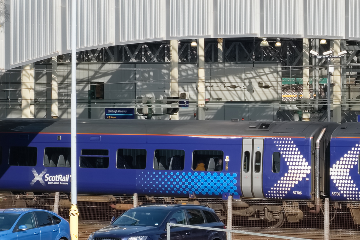
Train Detail..
Iridient X-Trans Demosaicing
Waverley Station, Single Image..
Car Detail..
Crane Detail..
Clock Tower Detail..
Train Detail..
25 Image Blend Results
200% Lightroom Demosaicing
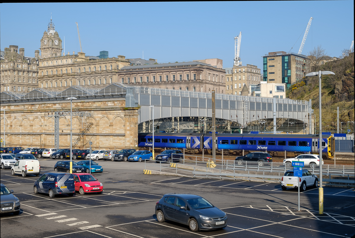
Waverley Station, Single Image..
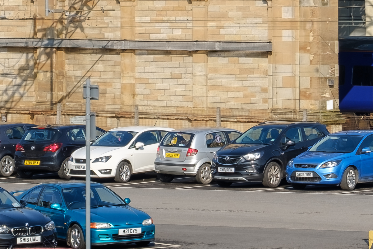
Car Detail..

Crane Detail..

Clock Tower Detail..
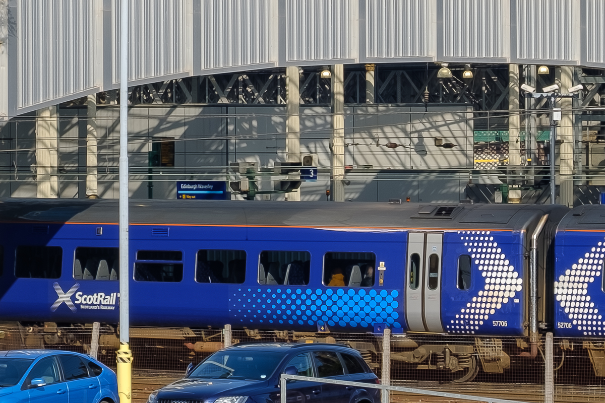
Train Detail..
200% Iridient X-Trans Demosaicing
Waverley Station, Single Image..
Car Detail..

Crane Detail..

Clock Tower Detail..

Train Detail..
400% Iridient X-Trans Demosaicing

Waverley Station, Single Image..

Car Detail..

Crane Detail..
Clock Tower Detail..
Train Detail..
15 Image Blend Results
200% Iridient X-Trans Demosaicing

Waverley Station, Single Image..

Car Detail..
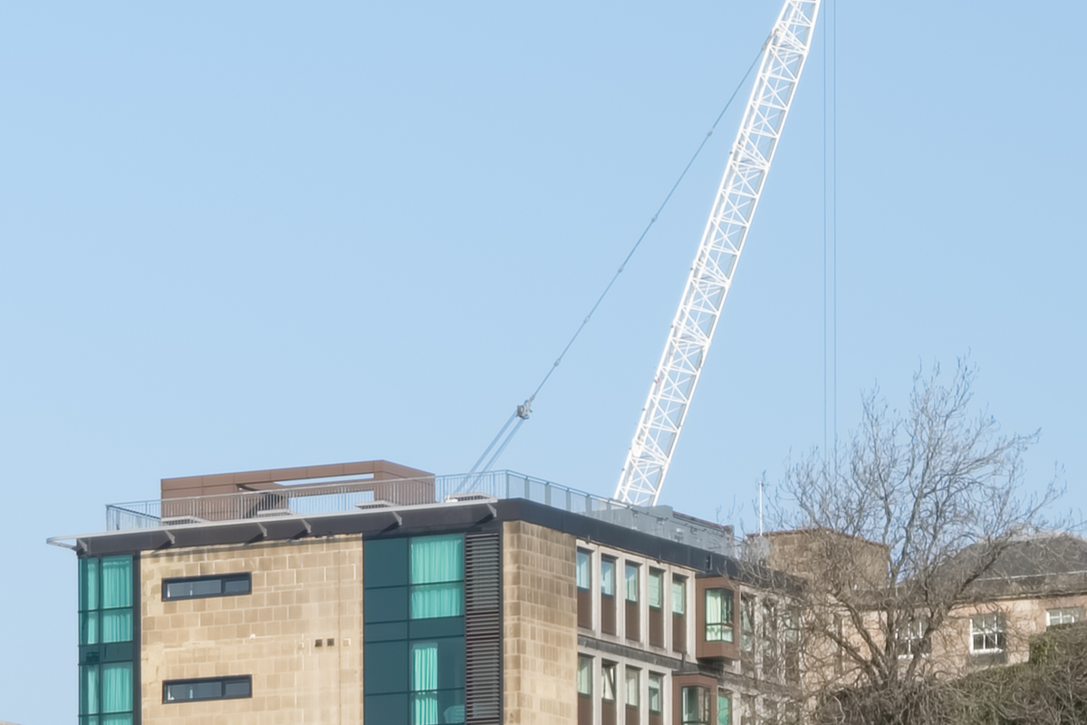
Crane Detail..

Clock Tower Detail..

Train Detail..
400% Iridient X-Trans Demosaicing

Waverley Station, Single Image..

Car Detail..
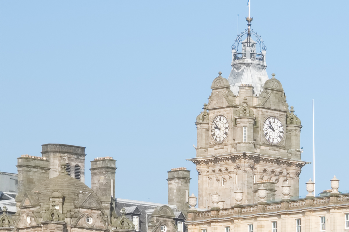
Clock Tower Detail..

Train Detail..
10 Image Blend Results
200% Iridient X-Trans Demosaicing

Waverley Station, Single Image..

Car Detail..

Crane Detail..

Clock Tower Detail..
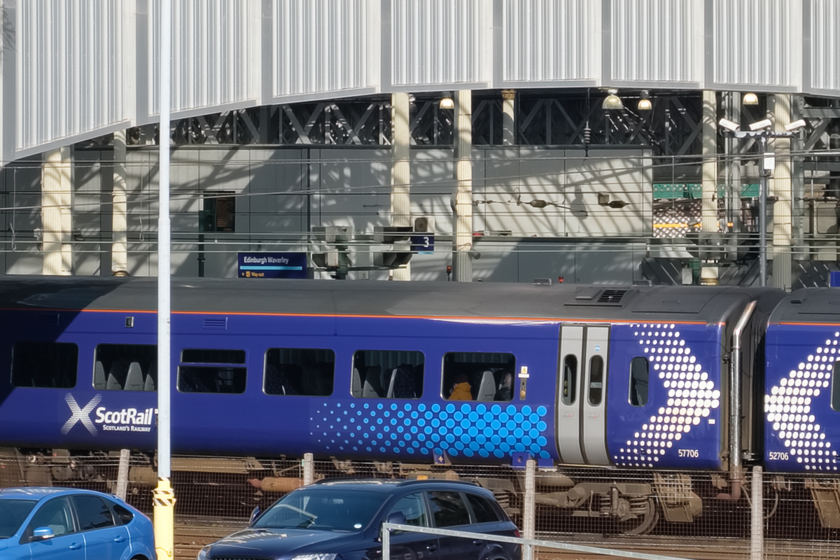
Train Detail..
400% Iridient X-Trans Demosiacing
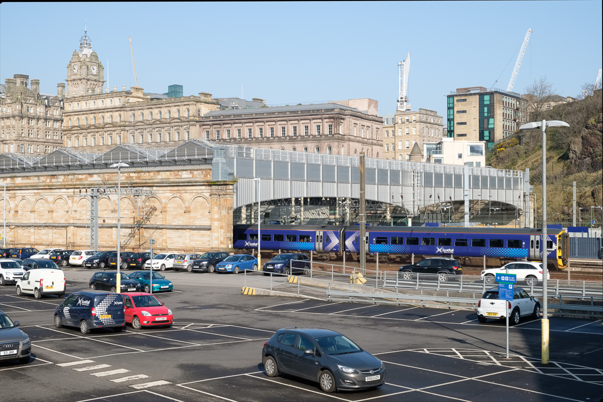
Waverley Station, Single Image..
Car Detail..

Crane Detail..
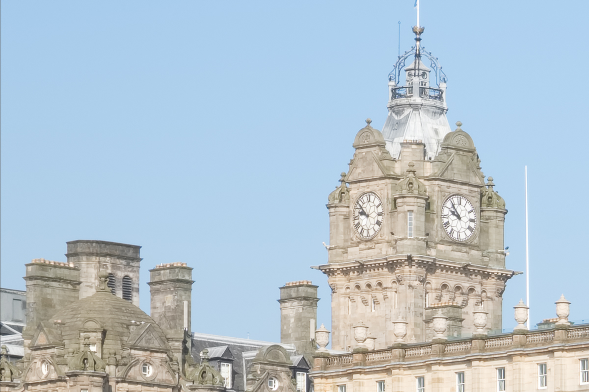
Clock Tower Detail..

Train Detail..
5 Image Blend Results
200% Iridient X-Trans Demosaicing

Waverley Station, Single Image..

Car Detail..

Crane Detail..
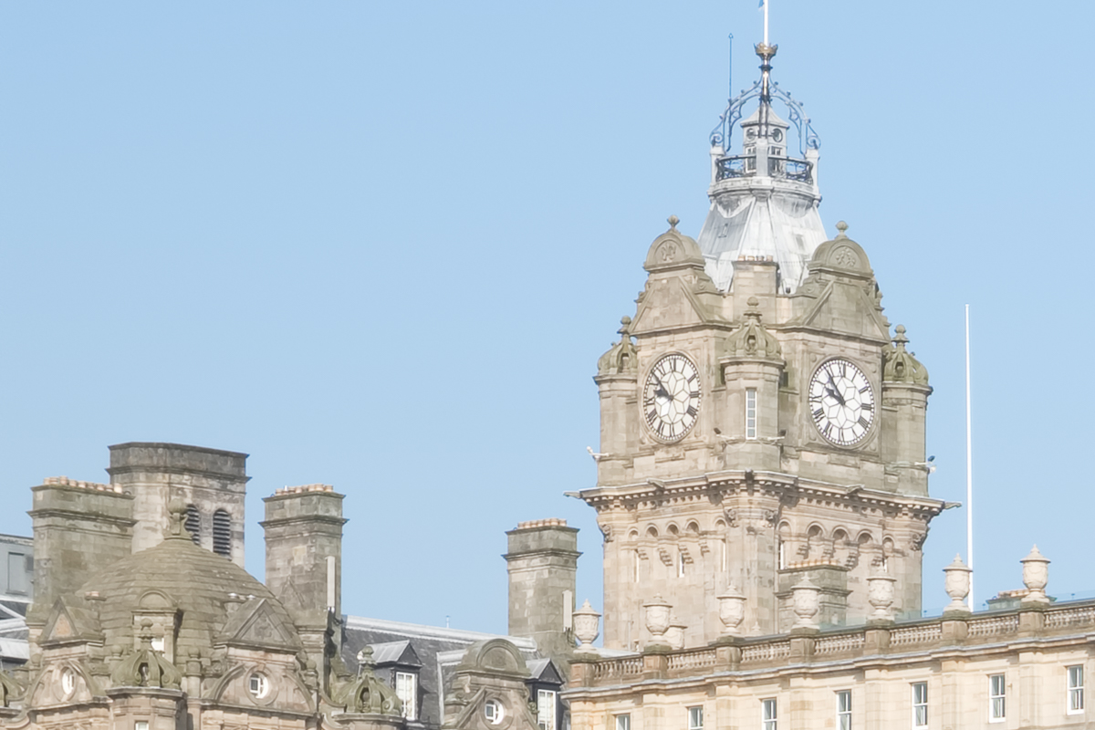
Clock Tower Detail..

Train Detail..
400% Iridient X-Trans Demosaicing
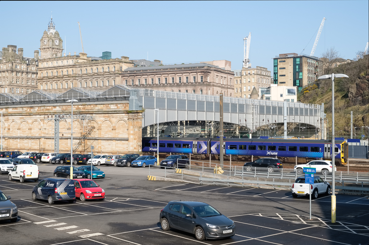
Waverley Station, Single Image..

Car Detail..

Crane Detail..

Clock Tower Detail..
Train Detail..
Summary of Image Findings
Lightroom versus Iridient X-Trans Demosaicing in the Single Image Test
In this test, the first observation is that the Lightroom processing gave a darker result than the Iridient X-Trans did. Looking carefully at the individual images, the detail in the Iridient rendering is very slightly better with less aliasing and more pleasing colour in the overall image. Moving on to the single image detail shots, it is very clear that the Iridient Demosaicing is superior. There is a noticeable level of extra detail with the images looking sharper with an oveall sheen and sparkle missing from the lightroom images which look muddy in comparison.
25 Image Blends at 200%
In the overall Waverley image there was again a difference in colour between the lightroom and Iridient X-Trans renderings with the Iridient looking more pleasing with better contrast and slightly less harsh aliasing. There was less false colour though the detail was fairly similar to my eye.
Comparing the Lightroom single image to the Lightroom 25 image blend there is a very noticeable increase in the clarity of the image. The car detail images have a sparkle to them that was missing in the individual rendering and the extra details in the car number plates and the chain link fence behind the cars is remarkable. There was little noise in the original Fujifilm XT-20 raw files which were taken at an ISO of 200, but the 25x image blends are totally noise free.
Comparing the Lightroom blend to the Iridient blend, there are further gains in image resolution and quality, to me most noticeable in the appearance of the chain fence where it overlaps the train wheels in the train detail image. The similarity of the colour of the rusty chain link to the false colour shadows under the train in the Lightroom image makes the link much more difficult to see in the Lightroom image.
25 Image Blends at 400%
I think that the key question here is whether there is any extra detail at all in a 400% size image compared to the 200% images. Here we are comparing simply between Iridient X-Trans demosaiced image blends only as I did not perform the 400% blends using a Lightroom render for reasons of time (more on the time aspect later).
To my eye, the 400% results were softer with less contrast, but noticeably less aliased and artefacts were fewer around small details like the number plates in the car detail image. It looked as though the 400% images might respond really well to a mid-tone contrast boost which may reveal this extra detail more clearly. The 400% 25 image blend took six and a half hours to render (after many failures to complete and certain tweaks being necessary to my computer hardware). As such the small gains may not be worthwhile as a routine workflow.
Reducing the Number of Blended Images
Reducing the number of images from the 20s to the teens may improve the speed of processing considerably, but is the lost quality acceptable. How many images do you really need. Ian Norman likes to use about 20 images which clearly works well, so I have started from 15 images working down in 5s.
Looking particularly at the Car Detail shots at 200%, there is an improvement in detail above that of a single shot even with 5 images. The improvements in detail and contrast improve incrementally the more images you add. 15 images is quite acceptable, though 25 gives a surprising amount of extra contrast and detail.
Going through the same exercise with the 400% images there is much less difference in contrast and detail as you increase the number of blended images. At 400% even 5 blended images gives a substantial increase in detail over the single image, so given the time in processing there may be little advantage in going to much larger frame numbers.
Practical Difficulties with Super-Resolution
With a 24 mega-pixel camera sensor, at 200%, you are essentially creating a 96 mega-pixel image (12,000 x 8,000 pixels). With a 400% super-resolution image you are creating a 384 mega-pixel image (24,000 x 16,000 pixels). Each 24 megapixel layer in your super-resolution stack will be 137 megabytes in size at 100%, so for a 25 image stack that’s 25*137 megabytes. Increase to 200% size and this becomes 25*549 megabytes file size or at 400% size a massive 25*2.15 gigabytes.
Needless to say that these file sizes are problematic for Photoshop to work with. It can do it, but it needs a massive amount of memory to do so. Way more memory than an average domestic PC will have.
Out of Memory?
I have a decent specification PC even though it is now a few years old (see link). But I was unable to process 400% super-resolution images with 25 layers because I kept getting out of memory messages half way through. It took a while to work out precisely which memory was running out, but it turned out to be both the Photoshop scratch disk and the Windows page file.
Of Scratch Disks and Page Files..
My PC uses a 500 GB M.2 SSD for the operating system and programs and, by default, Windows uses the operating system drive for its virtual memory management. Photoshop also uses the operating system drive for its scratch disc. Basically, my C: drive was filling up with virtual memory files and grinding to a halt. As good fortune would have it, I have a second, empty, high speed M.2 drive in my system so I was able to relocate both the Windows page file and my Photoshop scratch disc to that 500 GB drive. Sadly that still wasn’t enough space for these gigantic files and I had to add slower hard-drive capacity to the Photoshop scratch disc list after which all was well. Nevertheless, having had to wait six and a half hours for photoshop to finish, I only ran one 400%, 25 layer, file through the process. This is definitely a major limiting factor.
Is Super-Resolution Worth Doing?
My analysis is that it is worthwhile for some types of imagery:
- When you are in a push, especially in situations requiring high ISO to reduce noise as well as improve detail.
- For architecture and some indoor shots.
- For landscape photography in calm weather.
- In situations where you might want to make a very large print.
- When you don’t have a high resolution camera available, or where resolution stitching is not viable because you don’t have a long lens handy.
- In situations where extreme upscaling is necessary (400%) the availability of 5 images or more for this process gives a significant lift to the detail of the image.
Nevertheless there are situations in which you couldn’t use the technique, for instance where there was a lot of movement in the scene, or where every image is substantially different. Notwithstanding this some authors have used long-exposures for blurring water with this technique, so in some circumstances movement per se may not be an absolute barrier. It may also be used where small changes in perspective mean that the images can still be aligned (although there will be more waste within the image).
Final Thoughts
Iridient X-Transformer does not respect the Lightroom processing settings, but does use the in-camera film simulation. I would have been better off not making any development changes in Lightroom to ensure that judgements of the differences in resolution and contrast were not colored by them.
Feb
15
Uni-White Balance on a D850
How Much Difference Does it Make to Assessing ETTR?
I’m very much in favour of using an ETTR (expose to the right) methodology with all my RAW shooting. Uni-white balance is a way of improving the exposure information from your on-camera histogram, which is based on the jpeg processing currently in force when you take your shot. This jpeg processing, in turn, is determined by the picture control that you have selected in-camera. Setting a neutral picture control, with flat contrast and zero sharpening, is itself a way to improve the accuracy of the in-camera histogram, because it limits extra white point and black point clipping. Unfortunately this only takes you so far. A larger difference can be made by using, so called, uni-white balance. But how much difference does this make in practise, and crucially, is it useable?
What is Uni-White Balance?
Background
Checking the histogram and the clipping information is part of everyday routine for many photographers. Sadly the histogram and clipping information (blinkies) do not closely relate to the information captured in a RAW file. This is because the histogram is taken from a version of the JPEG file that the camera produces (stored inside the RAW file). The correlation between the information in the JPEG file and the RAW file depends upon the modifications that occur during the processes of:
- White Balance
- Application of a Contrast Curve
- Colour Profile Conversion (sRGB, Adobe RGB)
- Gamma Correction
- User Chosen Picture Controls or Settings (Contrast, Saturation, Sharpening etc)
These changes frequently lead to a pessimistic assessment of what the RAW file actually contains, leading to apparently blown out highlights for channels that are not really fully saturated in the RAW data.
In Camera Histograms
It’s difficult to know, for certain, exactly how the in-camera histogram (prior to the shot being taken) is really calculated. What may be happening is that the histogram that you see is derived from only a part of the image processing chain that produces the JPEG file. In live view it is likely that the camera sub-samples (to make the calculation faster) and assigns the pixels to buckets. To make the JPEG, the camera performs the additional 8×8 discrete cosine transform, file compression and formats the data in the nominated pattern for a JPEG file format. The histogram that you look at when viewing the file, post capture, is probably calculated from the JPEG preview file embedded within the raw file itself.
Almost always, the in-camera histogram, after this extensive processing, will not help you perform ETTR as it will show clipping at the right side of the image well before the raw data is actually clipped. Choosing the widest gamut camera color space (Adobe RGB usually) available, setting uni-wb and using the lowest contrast setting available (including removing any sharpening) will all help to give a closer approximation.
The RAW Image
The sensor in a Nikon D850 is covered with a so called colour filter array using a Bayer Pattern. Sometimes referred to as an RGBG pattern, the Bayer filter mosaic was invented by Bryce Bayer whilst working for Eastman Kodak in 1976. Colour filters are needed because the typical photo sensors detect light intensity with little or no wavelength specificity, effectively only measuring luminosity rather than colour.
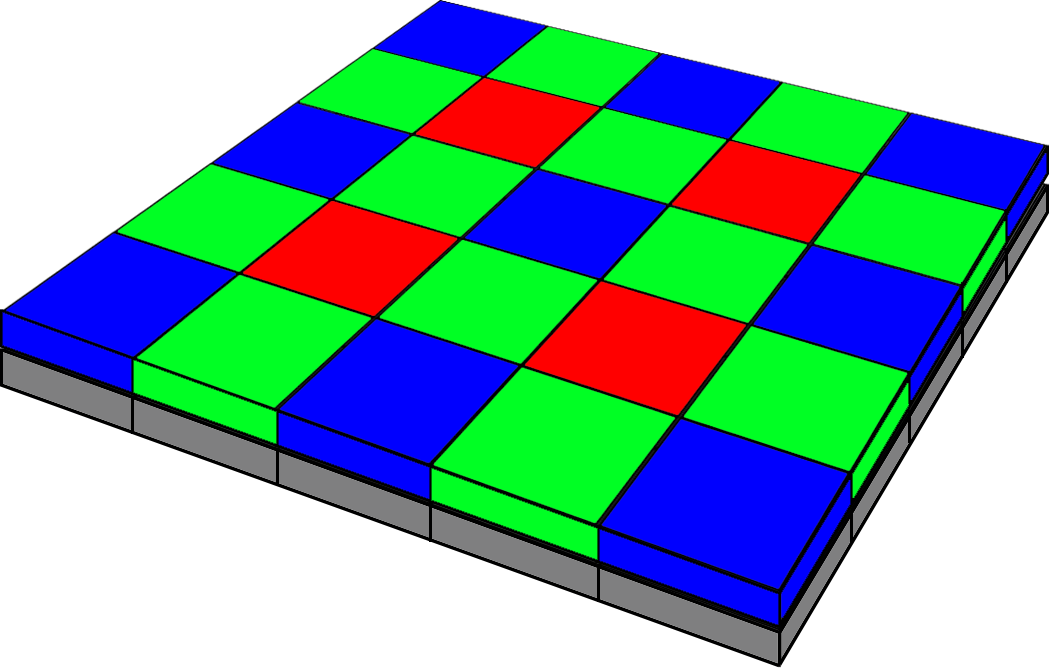
Bayer Array
With a colour filter array in place, a calculation can be performed for each pixel to work out its precise colour based on its own colour and intensity, alongside those surrounding it. This is called demosaicing. The Bayer pattern has twice as many green filters as red and blue. The colour filter’s spectral transmission, and density, will vary between manufacturers and need to be taken into specific account during the demosaicing process and translation into an absolute colour space.
The extra green filters provide more luminance information, which mimics the way that the human eye fabricates the sharpest possible overall colour image. In other words the human eye sees luminance and grayscale better than it does colour, and luminance better in the greens.
Demosaicing
Demosaicing is the process of turning the raw sensor information into an RGB colour map of the image. Various algorithms exist for this process though, in general, slight blurring takes place as a result of the demosaicing process. Some algorithms try to take edge detail more into account in order to mitigate the overall colour averaging process that takes place over groups of pixels. In order to calculate the red, green and blue values of each pixel (i.e. the missing two thirds as only the red or green or blue value is measured for the index pixel according to it’s colour filter), the immediate neighbour non-index colours surrounding that pixel can be averaged. Thus, in some sense, the colour map is two thirds fabricated and only one third measured!
Conversion to a Standard Colour Space
The raw data is not in a standard colour space, but can be converted to one later. As such, it does not matter what you set your camera to (Adobe RGB or sRGB) because the raw data is preserved with the colour space setting representing merely a label. The details of conversion from raw data to a standard colour space contain many complications. For a start a camera sensor is not a colorimeter so it is not measuring absolute colours anyway. You may hear this stated as camera sensors ‘not satisfying the Luther-Ives or the ‘Luther-Maxwell condition’. Secondly, human eyes and colour filter arrays see different spectral frequencies which can lead to camera metamerism. Camera metamerism is a term that covers the situation in which there is a discrepancy between the way a camera and a human sees colour. Typically colours that the camera sees as the same, which a human sees as different, or vice versa. Metamerism also occurs in printed output, especially with pigment inks. Jim Kasson’s excellent article on how cameras and people see color is a useful read for more information, as is John Sadowsky’s article on RAW Files, Sensor Native Color Space and In-Camera Processing.
White Balancing and the Green Coefficient
The next step of in-camera image processing is to apply the white balance. There are lots of ways to do this involving matrices and RGB coefficients. In this scheme the Green coefficient is set at 1 and the Red and Blue coefficients define the neutral axis of the image.
Final Steps in Camera Raw Image Processing
Finally, there will be the addition of a gamma correction to each of the 3 colour channels. In essence this correction takes account of the non-linearity of the human perception of tones and can also increase the efficiency with which we store colour information.
Uni-White Balance
The ‘uni’ in Uni-White Balance really refers to 1. That’s 1 as in a white balance in which the red, green and blue coefficients are all set to the same value (i.e. 1).
When a camera or post-processing software (RAW convertors) apply a white balance to the RAW data, they generally leave the green data as is and apply a factor (the coefficient) to the red and the blue channels. So, for example, at sunrise and sunset when you have an abundance of warm (red) light, the red is lowered and the blue increased.
On a cold overcast day, or in shade, the reverse occurs so that the red is increased and the blue lessened. This factor, or coefficient, is thus a divider or a multiplier of the actual raw data from the sensor for the red and blue pixels. This may therefore lead to either an underestimate or overestimate of how much red or blue channel saturation is really present. In other words the red and blue channels can look either under or overexposed erroneously compared with the actual values recorded in the raw data from each red and blue photosite.
Uni-White balance uses coefficients of 1 for red, green and blue which thus leads to accurate histograms and highlights for your raw data provided that any picture control (for Nikon) in force does not artificially boost saturation or contrast in one or more channels.
More on White Balance
As mentioned above, the white balance is the linear scaling of the RGB channels of the RAW file. This means that the levels of red and blue are typically multiplied by a factor greater than 1 which scales them to compensate for the different sensitivities of the filtered photosites, and also the colour of the light in the scene (eg. daylight, tungsten or shade). These linear factors can be as high as 2 or even 2.5 leading to an apparent increase in exposure for the channel being scaled from 1 EV to 1.3 EV. Similarly, decreases in exposure may also occur leading to desaturation of the image in some colours.
Setting up a Nikon D850
There are techniques that approximate to Uni-White Balance and techniques that are specific to a particular camera. Both are comprehensively covered in Jim Kasson’s ‘the last word‘.
Approximations to Uni-White Balance
The shortcuts to Uni-White Balance do not work on all cameras.
Balance to Maximum or Minimum Saturated Pixels
Taking a dark frame image (for instance with the lens cap on), or a completely overexposed and blown out image, as a reference for White Balance is one way to get the same information in all the channels. This will sometimes work for some Canon cameras, but doesn’t work for Nikons. To check whether you have achieved the desired white balance check the red and blue white balance coefficients in the camera’s EXIF data. They should be within five or ten percent of one.
Manual White Balance Technique
In this method you set the white balance to 3800k (or as close as you can) and then set the colour bias (or tint) to as green as it will go. Take test exposures and check the EXIF white balance coefficients as above. Use the manual white balance to tweak the settings but beware that many cameras just don’t have enough adjustment range to get you to a full Uni-White Balance.
Use a Uni-White Balance File Prepared for your Camera by Someone Else
In this method you copy the white balance setting from a copy of an image taken by another camera, of the same make and model, with Uni-White Balance already set up. Copy the image to a memory card (with a suitable name and in a suitable folder so that the camera can find it) and tell the camera to use the white balance coefficients from the image as a white balance preset.
Avoid Uni-White Balance and ETTR Using Another Method
If you are confident that you know what the brightest part of your capture will be, you can meter for that, apply +3 stops of exposure compensation, and not use the histogram at all.
Setting up a Specific Camera for Uni-White Balance
I have personally used the method described by Jim Kasson on his blog. Since you are also free to use this resource I will not précis it here, suffice to provide the link and make a few comments on issues that I found particularly challenging. In essence, the task consists of taking defocussed, fully saturated, pictures of red, green and blue on a fully warmed and calibrated monitor using (for instance) photoshop. A second program (I used Rawdigger) gives you the average pixel values of the Red, Green and Blue in the raw images so that these values can be entered into a spreadsheet that Jim provides. The spreadsheet gives you values for a corrective (magenta) colour which you create and display on your monitor. This colour is then used to white balance your camera and store a preset for future use.
As I traversed Jim’s excellent protocol, the only real question that I had was about whether to use exactly the same exposure for the White Balance as for the RGB target images. It turns out that it doesn’t really matter. It doesn’t really matter what the exact exposure of the RGB targets is either, you really can let the camera decide. Secondly, when it comes to entering the desired camera values in the spreadsheet, it does make a difference to the magenta target brightness values calculated (but not the hue) so again they are not critical. Finally, I calibrated 5 cameras in one session and found that it is quite easy to forget to enter the desired camera values. So keep an eye on that detail.
Side Effects
It goes without saying that success in this process leads to raw images with a heavy green cast (the background of this image was neutral gray). This is easily dispensed with by choosing an appropriate white balance preset in your image processor of choice, during post. After a while you stop noticing the cast and I tend to leave Uni-White Balance set most of the time.
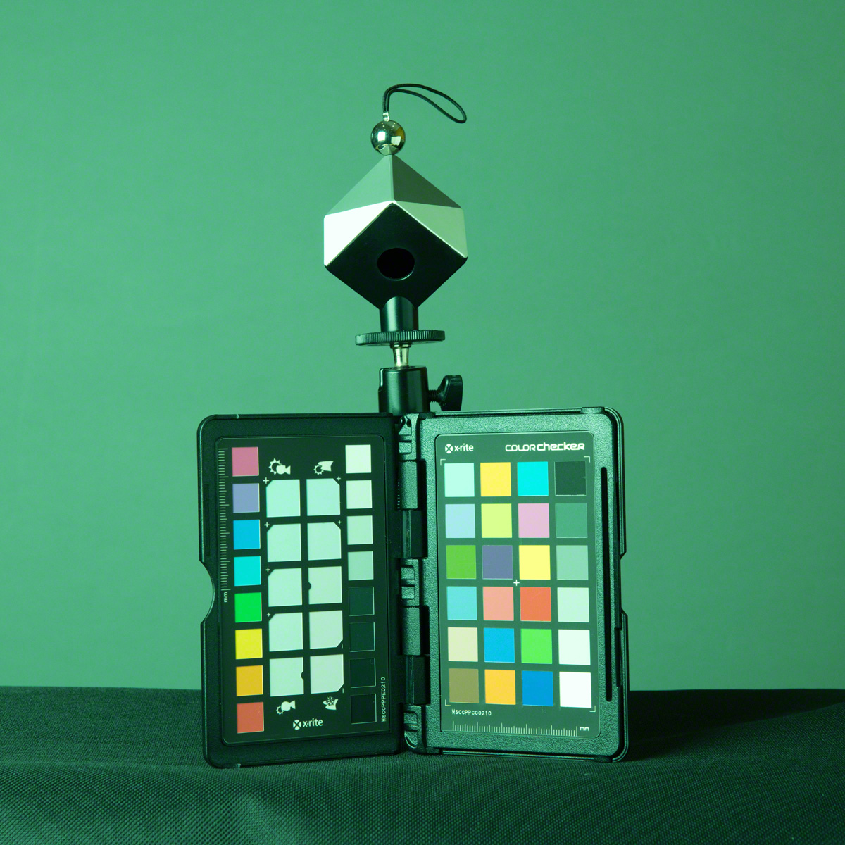
Image with Uni-White Balance Applied
Picture Control Settings
As mentioned previously I used the NL picture control preset but edited it to remove all sharpening. I left contrast at zero, though you could make it lower still. Just as an aside, Nikon makes the excellent Picture Control Utility 2 which comes free with other Nikon software or can be downloaded from the link included. This utility allows you to organise and manage your picture control presets so that they may be distributed between Nikon cameras. There are some features within the utility that are not available for adjustment in the camera picture control menus.
Testing the Effects
The Setup
My goal with this testing was simply to get a feel for how the histogram looks between shots taken with, in this case Auto White Balance, and Uni-White Balance across a range of exposures. To maximize accuracy I chose to use a manual flash exposure in order that there was no chance of the light levels changing between shots. I chose an exposure that meant the flash was the major lighting for the scene and no chance of the ambient lighting causing specular highlights. All shots were taken at 1/160th second at f11 and an ISO of 800. There is a debate to be had about which ISO to choose, but given that the D850 has an ISO invariant sensor, and that I’m often shooting wildlife in low light conditions, this seemed a reasonable compromise for this experiment.

Lighting Setup with Targets
As can be seen from the image at left, the target was an X-Rite Color Checker Passport beneath a Datacolor SpyderCube White Balance target. The advantage of the SpyderCube is that the metal ball atop creates clear specular highlights, and the dark face has a light trap within it to give a definite black point.
The colour in the scene comes from the Color Checker only, with everything else being neutral. You can see a small colour cast across the grey background in the production shot, but this is removed by the ambient under-exposure and flash illumination. There did remain a small luminosity gradient across the background however as a result of using only one softbox. This is partly mitigated by the V-Flat reflector and, not a significant confounding variable in this test. The camera was tripod mounted and did not move during the test shoot.
Testing Procedure
Below is an image of the ambient light at 1/160th second, f11 and ISO 800. The test itself consisted of making 10 exposures at 1/3rd stop intervals via a Nikon SB910 Speedlight set to manual exposure. The range was 1/8th power to 1/64th, chosen to be well within the normal range of the speedlight output (Full power to 1/128th). Shooting at a maximum of 1/8 power also provides insurance against the flash not being ready for the next shot. The flash was triggered using a Pocket Wizard Flex tt5 with a mini tt1 on camera alsongside the AC3 controller for easy and precise flash settings.
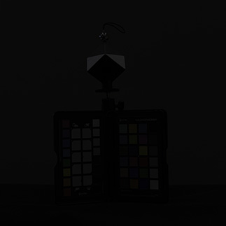
Ambient Exposure
The Nikon D850 was set to Raw shooting and a set of 10 shots using Auto-WB 1 were made (Light to Dark exposures) followed by 10 shots using the Uni-White Balance Preset (as above). Again, bright to dark exposures.
The 20 Raw Files were then inspected on the back of the camera and the histograms photographed. The Raw Files were brought into RawDigger and examined for highlight clipping in each exposure. These values were entered into a spreadsheet (see below).
Results
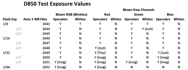
Auto-1 White Balance Data
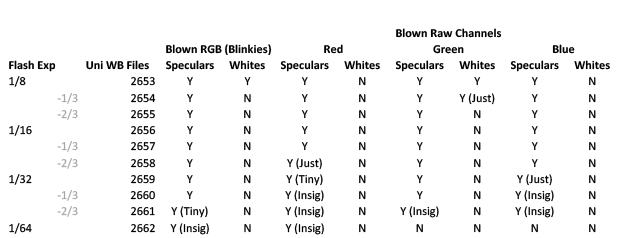
Uni-White Balance Data
The first thing to notice is that these tables are, barring one small detail (a tribute to Nikon flash consistency) exactly the same. In other words (and reassuringly) the exposure captured was not materially altered by the application of Uni-White balance.
Does this mean that the back of camera histograms are the same? Not at all! My first examination was to look at whole stop increments.
Composite Histogram Analysis
You can compare the histogram results to the RawDigger results by looking at the Hist No in the spreadsheet above (I.e. the number out of 208 in the images below).
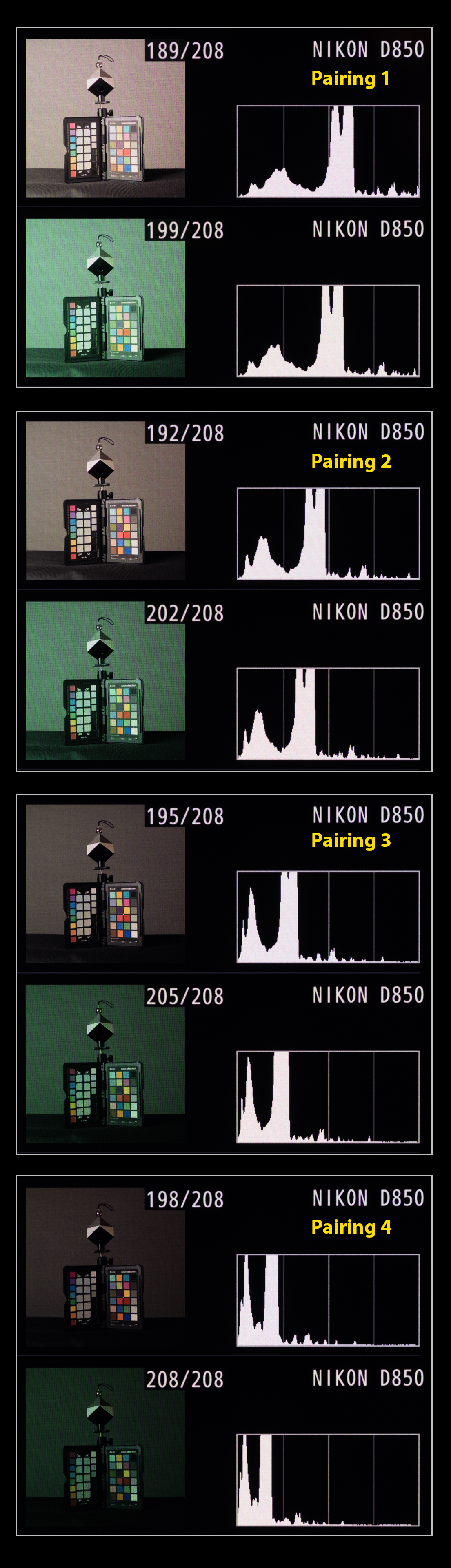
The graphic shows four images, one stop apart in auto and uni WB pairs. As you can see the Uni-WB composite histogram is consistently left shifted (demonstrating more exposure headroom) in the Uni-White Balance partner. It’s reasonably easy to compare the peaks between histograms. The horizontal movement of peaks between successive Auto-1 White Balance Composite Histograms gives a measure for a one-stop difference in exposure. Bringing the images into Photoshop and applying the measurement tool, it looks as though a stop measures about 228 units, on average. This being the distance between the same histogram peak between images, on a full sized image. Comparing this between successive Auto-1 White Balance / Uni-White Balance pairs shows a distance of 88 units on average and this represents a 0.39 Stop improvement in accuracy on the composite histogram.
RGB Histogram Analysis
The image below shows 4 RGB histogram pairs with each pair representing 1 stop exposure difference, decreasing down the page as with the composite histograms above. At first the picture seems very confusing. The inflated green channel (or perhaps I should say, the more representative green channel) looks at first as though it may be a problem. Looking at the RawDigger white clipping values for the Green channel though, as with the images of the on camera histograms below, you can see that this reduces at the same rate in both sets of files and looks worse than it is. Also, because the red and blue channels are also shifted, you still end up with a better composite histogram. For this reason, ease of interpretation may improve by just using the composite histogram whilst Uni-White balance is in place.
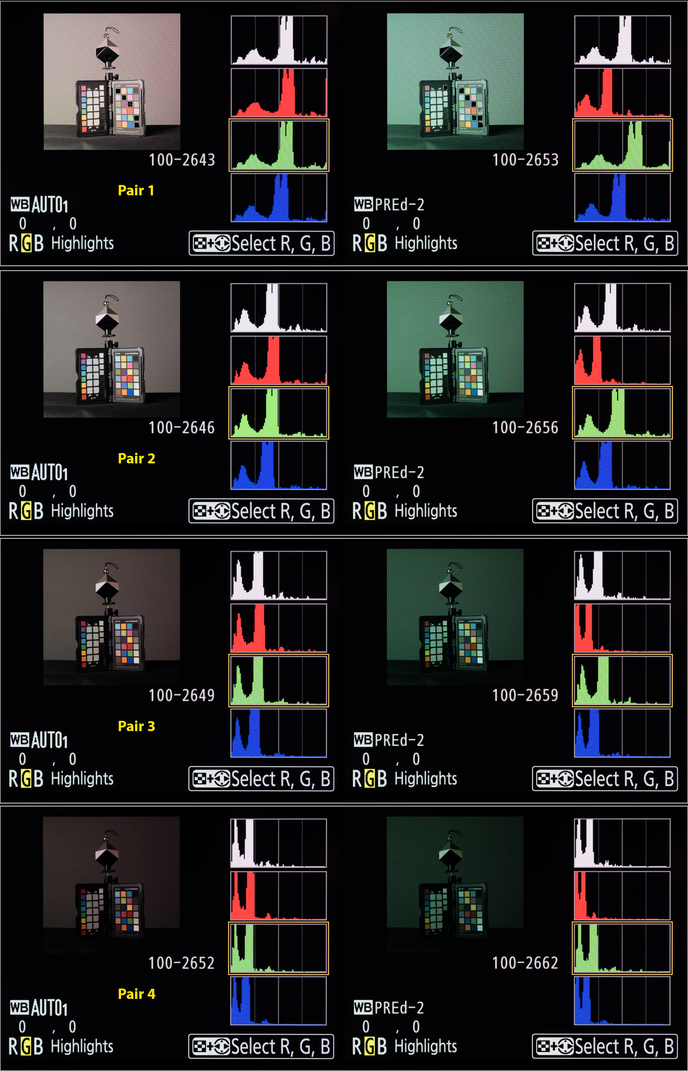
RGB Histogram Pairs, 1 Stop Apart
Usability In Practise
I am still gaining experience with this technique, though my initial impressions are good. I was worried that the heavy green cast would put me off using Uni-White Balance, though in practice this is not the problem I first thought. You stop noticing it after a while. I was also concerned about moving back and forth between the white balance presets, but on the Nikon D850 at least, you can lock the Uni-White Balance preset so that there is no chance of overwriting it by mistake. I have set mine in the second custom white balance slot in all my cameras in order that setting a different custom white balance is not hindered when not using Uni-White Balance.
In Camera Settings
In camera I set a flat picture profile (NL or Neutral in the D850) with sharpening reduced to the minimum possible. Although preferable to use the Adobe RGB colour space in camera, I choose to use sRGB. This is to counter the problem of forgetting to change any camera generated jpegs back to sRGB prior to using them on the web or social media. In this regard I believe the Nikon default setting of sRGB to be the most pragmatic though I concede there may be further improvements in accuracy to be made by swapping.
Post-Processing Uni-White Balance Images
I am still gaining experience with post processing Uni-White Balance images. Nevertheless, after correcting the white balance via an appropriate white balance preset, or by correcting using a neutral tone within the image, smaller changes to exposure than usual are my major finding to date.
Conclusions
Using Uni-White Balance gives a 0.39 stop improvement in accuracy on a Nikon D850 over and above that obtained by using a flat Picture Control. Interpretation of the green channel information in the RGB histogram may be hindered by the more accurate representation of the green channel in some circumstances, but the more accurate rendition of the composite histogram reduces the risk of relying solely on the composite histogram.
References

Oct
06
Turn a White Background Black
Really, Are You Having a Laugh??
I’ve watched several YouTube videos on taking pictures in adverse circumstances, including how to turn a white background black. Have you ever tried this yourself? It may not be as easy as you are made to think.
The Basic Principles
Underexposing for Black..
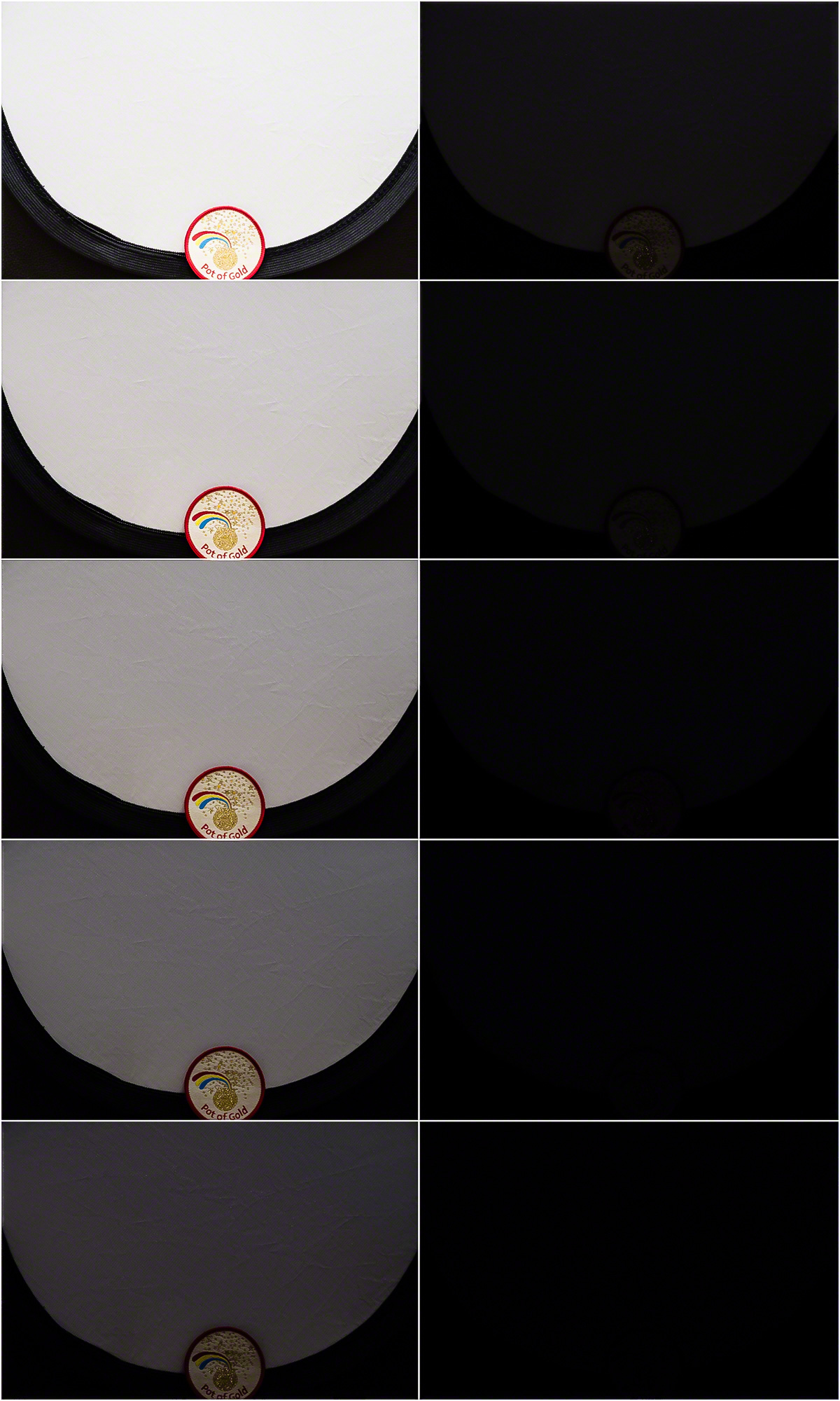
In order to turn a properly exposed, non-clipping, bright white background to black it will need to be under-exposed. How much may depend on the contrast of the light used and the reflectivity of the surface, but is likely to be between 6-8 stops. In the example at left, the bright white, non-clipping exposure was 1/4s at f5.6 and ISO 400 whereas the dark exposure was 1/500s at f5.6 and ISO 400, some 7-stops less.
The chart at left shows the incremental reduction in exposure, one stop at a time, of a small white Lastolite reflector. Although, at a distance, a 5 stop reduction looks adequate, you can clearly see the reflector in the image on the computer.
The ambient exposure needs to be reduced substantially in camera, and the subject re-illuminated, to compensate for the reduction, usually with flash. Shooting in manual, most flashes have a range of 1 to 1/64 or 1/128 power (6 or 7 stops respectively). This may sound a little close for comfort (which it may be), especially when using light modifiers that reduce the flash by 2+ stops. You can also place the flash nearer to the subject if needs be however.
What Can Go Wrong?
When trying to turn a white background black, the re-illumination of the subject has to be specific to the subject. In other words, the 7 stops of flash that you add back in must not travel to the background and re-illuminate it as well! This is awkward in smaller studios (or a mostly white painted kitchen as in this case) where flash bounces round the room increasing the ambient again.
Mitigating The Re-Illumination Light Spill
There are two main ways of managing light spill, firstly to manage the direction of the subject re-illumination light (so that it misses the background) and secondly using the inverse square law in setting the flash to subject and subject to background distances. In the smaller studio it may also be necessary to mitigate bounced spill by using flags or black reflectors or covers.
Managing Light Direction and Spread
Two main strategies will help here. Firstly, avoid front lighting if you can because the spill will necessarily hit the background. Try and use side lighting or lighting from high up and to the side so that the spill-light travels past the side of the background or down to the ground. Secondly, use light modifiers to narrow the direction of light rather than having light going off in all directions. Choose your modifier based on the following priority list (worse to better) for best directionality.
- Shoot through umbrella
- Bare flash with wide spread
- Shoot back umbrella
- Bare flash with narrow spread
- Softbox
- Deep Softbox
- Softbox with grid
- Grid Spot
- Snoot
Finally, you may need to control spill by reducing reflections from large reflective surfaces. This can be achieved by using large black panel reflectors (or non-reflectors) or covering with black sheets or a roll of black paper. Obviously, if you have these to hand, I have to question why you are trying to turn a white background black in the first place!
Inverse Square Law
What is it?
What is the inverse square law, and how does it help? Basically the inverse square law states that the intensity of light from a source falls off with the square of the distance from the light source. So if the intensity of light is X at 1m from a light source, at 2m it will be X/4 and at 3m it will be X/9 and at 4m X/16. This has some interesting implications for the photographer. Firstly it means that every doubling of distance from the light source delivers a 2-stop fall in light. So, for an example, if you had a subject lit by flash at 0.5m then at a background set at 4m there would be a reduction of 6 stops of light, and at a background set at 8m an 8-stop reduction. A small increase of flash to subject distance from 0.5m to 1.0m doubles the necessary flash to background distance to get the same reduction in light (namely 8 and 16m respectively – better order your new kitchen extension now!!).
How is it Used?
Secondly, and perhaps rather confusingly, the proportional light fall off with distance is greater close-in than it is far out. This is because the light intensity is the reciprocal of the distance squared so that, for larger distances, the difference between the fractions is necessarily less than for shorter distances. So light intensity at 2m is a quarter that at 1m, ie a 3/4 (0.75) reduction between 1m and 2m. At 4m the light intensity is 1/16 reducing to 1/25 at 5m. So the difference in intensity between 4m and 5m is 9/400 (0.0225). This is useful where subjects are at different distances from the flash. Moving the flash back to say 5m from the subjects would mean that there was virtually no difference in illumination between subjects at 4m or 5m (for instance in a wedding group shot).
Other Confounders
Managing light spill can be harder where you have, for instance, a white tiled floor, or a low white ceiling. The floor can be covered in extremis (beware the trip hazard though) but there is very little you can do to mitigate a low white ceiling.
Production Images and Results
Here is the setup for this shoot. You get some sense of the restricted space and can see the camera, subject and strobe positions clearly.
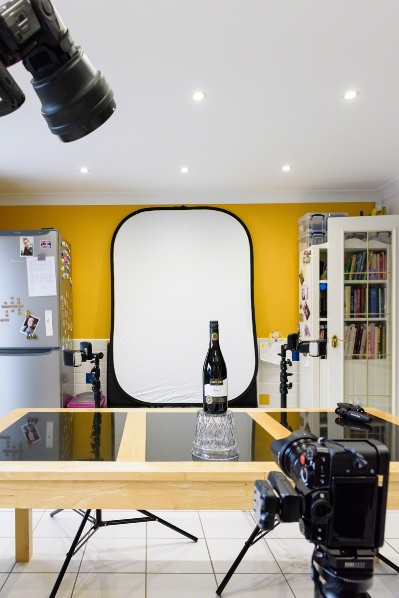
Kitchen Studio..
Post Processing
The three wine bottles shown below were all straight off the camera card and, apart from a small crop, completely unedited! So I’d have to say that the morning spent trying to turn a white background black was a complete success. I’m bound to also say, though, that I’ve no intentions of abandoning my beloved black velvet Lastolite panel background anytime soon.
Equipment Used
Equipment used was a Lastolite large panel Black/White reversible background, a Lastolite black velvet background to control spill (out of shot), 3 x Nikon SB900 Speedlights, 3 x Bowens Light Stands, assorted cold shoe clamps to attach the Speedlights to the light stands and a Gary Fong Collapsible Snoot with Power Grid for the key light. For convenience I was using 3 x Pocket Wizard Flex-tt5 radio triggers, with the mini-tt1 and AC3 controller on the camera. As you can see there is much white and silver in this room to bounce spill light around. The main kitchen lighting is daylight balanced and camera left sits a large kitchen window and patio door.
Camera and Flash Settings
The eventual camera settings were ISO 200, f11, 1/125s. The key light was set to full power and the rim lights adjusted to give a pleasing result at a much lower power (around 1/32).
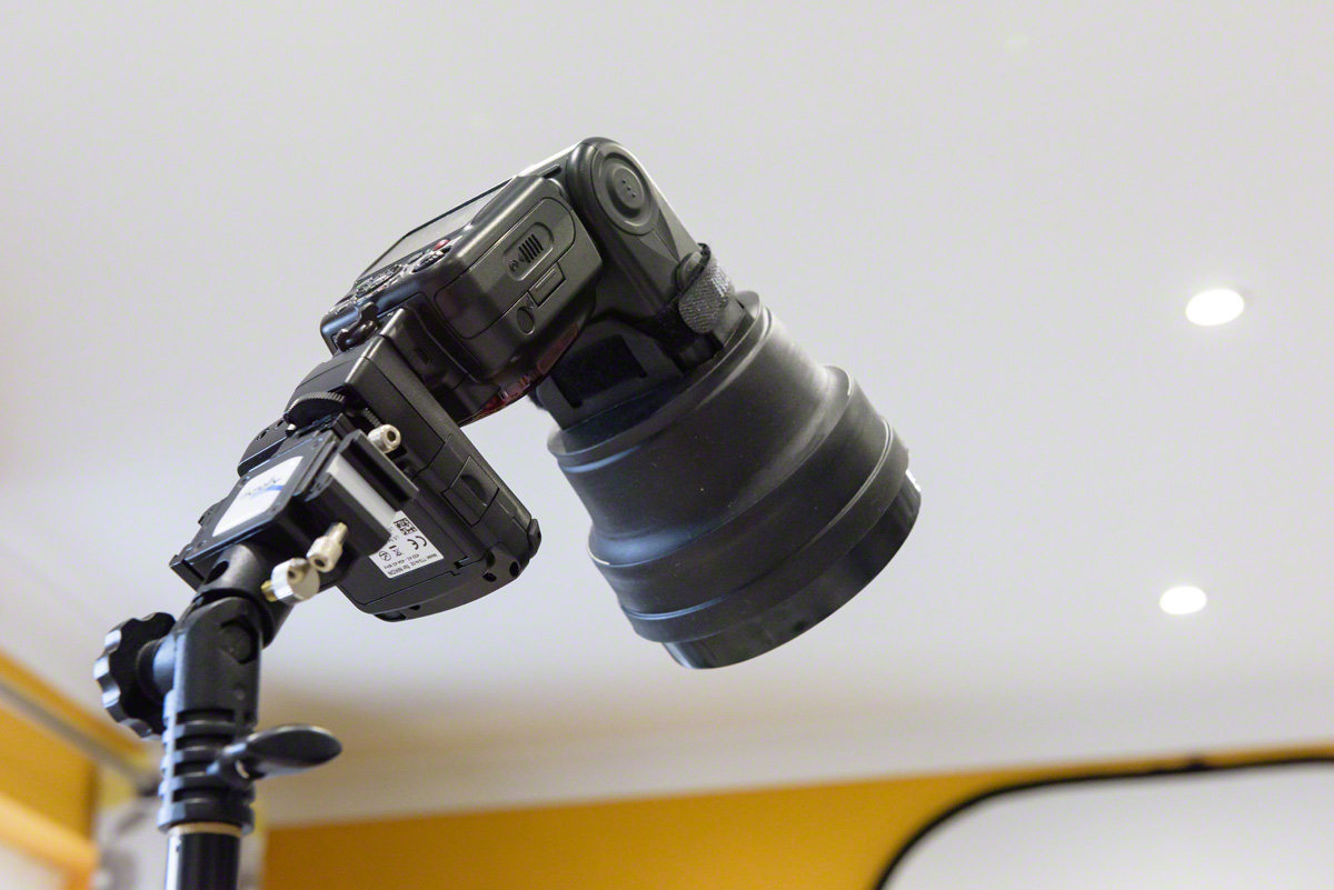
Key Light with Grid Fitted..
Use of the kitchen studio was only possible in the absence of other family members, so thanks also to them for leaving me with the house for the morning too. I think that it must be so lovely to have a permanent and dedicated studio where you are not hunting round the house for your equipment because it is all in one place. Or having to move chairs and furniture to create sufficient space. Perhaps when I retire.. You can only dream I suppose..
I feel a large man-shed coming on..
Final Thoughts
Small Kitchen Woes..
To pull this off in my kitchen studio I had to use all available space and had to keep the subject size down as I was rammed against the range cooker. You can’t see it in the production shot, but I had to manage some light spill with a large black panel reflector out at camera right. For me this was a technical exercise, just to see if I could do it. I have tried without success previously as I could not manage the light spill effectively enough. The subject to background distance, for me, was only about 3m so control of light spill was essential as I couldn’t afford to only rely on the inverse square reduction.
Controlling the Spill..
If I had needed more control of light spill, I would have thought about reducing the light from the white floor tiles and used flags on the rim light flashes to stop light getting onto the ceiling. Finally it might have been necessary to use another black panel reflector on the wall behind the camera to further reduce spill.
Could do Better..
As a technical exercise, I have added to my own difficulties by using my Fujifilm XT-20 travel camera instead of my Nikon kit. I don’t have a full flash setup dedicated to this camera system so I was working with manually. I was, however, very pleased to find that my flex-tt5s and SB900s could be used on my Fujifilm XT-20, controlled by the flex-mini tt1 and AC3 controller combo on camera in the usual way. The only concession was that I had to drop the shutter speed on my XT-20 to 1/125s in order to get reliable syncing. The XT-20 maximum sync speed is 1/180s which I am confident would have worked ok with optical syncing, but didn’t with the radio kit. Since my Flex kit is for the Nikon, I’m pleased that I was able to use it on the Fuji at all, so this was a small sacrifice to make.
Cheers,
R.
Recent Comments